
At the last EGSIEM project meeting (held in Potsdam, Germany in June), Zhao Li (of the University of Luxembourg) reported that she had problems calibrating the positions of GRACE A and B satellites when introducing K-Band observations. After some extremely helpful discussions with Uli Meyer, Adrian Jäggi, and some hand holding by Matthias Weigelt (BKG - Bundesamt für Kartographie und Geodäsie) Zhao went back and checked the code step by step. After two months of extreme frustration, Zhao is now extremely happy and satisfied that she has found and solved the problems. Now she gets a reasonable GPS/KRR combined reduced-dynamic orbits for GRACE A and B for the test date 01/01/2006. This means that we are getting closer to our final target.
During our orbit determination, we followed the Celestial Mechanics Approach (Beutler et al., 2010). The top two panels of Figure 1 give the difference between K-Band range rate (KRR) and range rate from GRACE A and B before and after combined GPS/KRR adjustment. The bottom two panels show the difference with respect to the kinematic positions of GRACE A and B provided by TU Graz. We can observe that the relative position between A and B are significantly improved after introducing KRR, and also the absolute position variations of A and B are at the reasonable level of several centimeters.
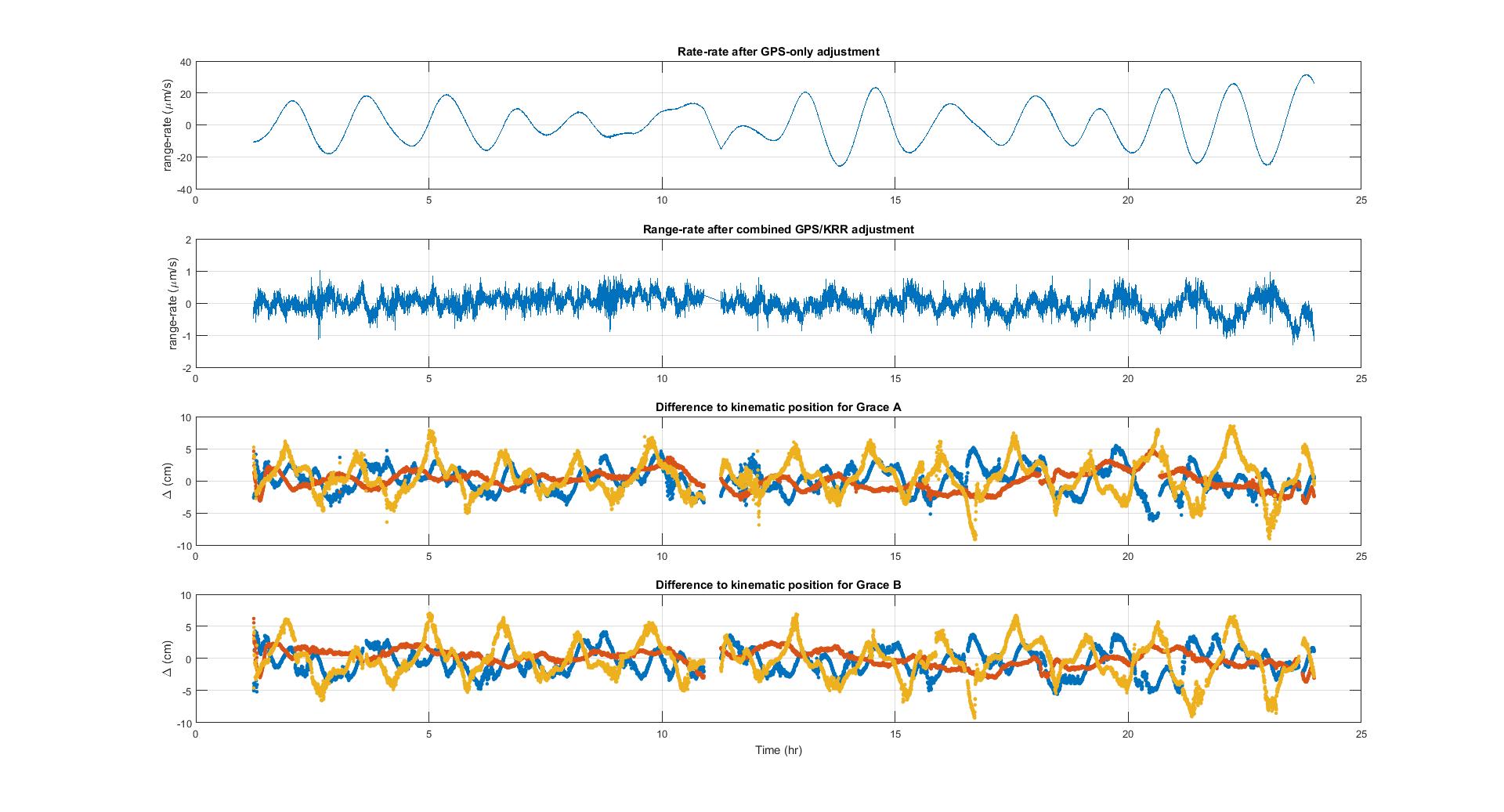
Figure 1. Combined GPS/KRR adjustment results
The left panel of Figure 2 illustrates that the residuals after combined adjustment are about two orders of magnitude smaller than our GPS-only orbit adjustment result (from top to bottom are b-b0, Ax and b-b0-Ax), which confirms that our combined adjustment works. Further, the right panel of Figure 2 shows the difference of Ax and the integrated difference (from top to bottom are b0new-b0, Ax, and b0new-b0-Ax). The results in this figure indicate that our integration is also problem free.
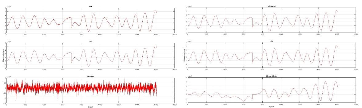
Figure 2. Range rate linearization error (Left: adjustment. Right: Integration.)
From Figure 1, we can also see that the difference between KRR and range rate from A/B becomes larger at the end of day, irrespective of whether the combined adjustment is applied or not . This result may be caused by the drift in the range rate, since we did not estimate this term during our set up. In the coming days, Zhao will continue to improve our orbit result by adding parameterization. Christian has provided her with their force model and GPS/KBD orbit on the test day weeks ago. After he found the GPS only orbit, Zhao could perform the orbit validation quickly. At the same time, Zhao has begun the next step in the implementation of the rigorous acceleration approach. ULUX is still behind. But anyone who knows Zhao knows that she will do her best to catch up with the other groups to provide ULUX's gravity solution as soon as possible.
And now for something completely different… We post a photo of Zhao’s son, Moxuan. He is very fond of Zhao’s laptop, and he will be generating gravity solutions in no time.

The celestial mechanics approach: application to data of the GRACE mission, Beutler, G., Jäggi, A., Mervart, L. et al. J Geod (2010) 84: 661. doi:10.1007/s00190-010-0402-6